Deploying a custom object detector on edge NPU hardware invovles training, quantization, and compilation. This guide walks through the entire pipeline using a YOLOv8s model trained on handwritten digits.
Training the Custom YOLOv8s Model
Preparing the Custom Dataset
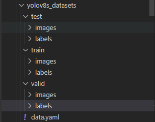
The dataset structure can be organized in any way; the following layout worked well for this example. A typical VOC structure is also acceptable.
digit_detection_data/
├── test/
│   ├── images/   # image files
│   └── labels/   # label files
├── train/
│   ├── images/
│   └── labels/
├── val/
│   ├── images/
│   └── labels/
└── dataset_config.yaml
The dataset_config.yaml file used in this project:
train: ../train/images
val: ../val/images
test: ../test/images
nc: 10
names: ['0', '1', '2', '3', '4', '5', '6', '7', '8', '9']
Setting Up the YOLOv8 Training Environment
Follow the official YOLOv8 environment setup:
# Clone the ultralytics repository
git clone https://github.com/ultralytics/ultralytics

# Navigate to the cloned directory
cd ultralytics

# Install the package in editable mode for development
pip install -e .
Download the pre-trained weights:
wget https://github.com/ultralytics/assets/releases/download/v0.0.0/yolov8s.pt
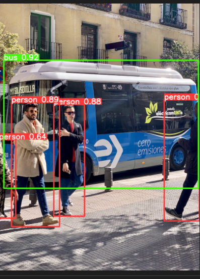
Verify the environment with a quick test:
yolo predict model=yolov8n.pt source='https://ultralytics.com/images/bus.jpg'
Training the Custom YOLOv8s Model
YOLOv8 supports training via CLI or Python scripts. We'll use a Python script for training and CLI for later testing.
cd ultralytics
Create a training script, for example train_digits.py:
from ultralytics import YOLO

model = YOLO('/root/ultralytics/yolov8s.pt')
model.train(data='/root/ultralytics/digit_detection_data/dataset_config.yaml',
            epochs=100,
            amp=False,
            batch=8,
            val=True,
            device=0)
Run the script:
python3 train_digits.py
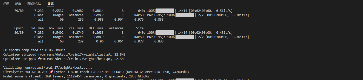
Test the trained model on a sample image:
yolo predict model=/root/ultralytics/runs/detect/train17/weights/best.pt source='/root/ultralytics/ultralytics/assets/digit_sample.png' imgsz=640

Model Deployment and On‑Board Testing
Preparing the Tools and Files
Exporting an ONNX Model for Pulsar2
Export the best checkpoint to ONNX with opset 11:
yolo task=detect mode=export model=/root/ultralytics/runs/detect/train17/weights/best.pt format=onnx opset=11
Simplify the ONNX graph:
python3 -m onnxsim best.onnx digit_yolov8s_sim.onnx
Simplification report:
┏━━━━━━━━━━━━┳━━━━━━━━━━━━━━━━┳━━━━━━━━━━━━━━━━━━┓
┃            ┃ Original Model ┃ Simplified Model ┃
┡━━━━━━━━━━━━╇━━━━━━━━━━━━━━━━╇━━━━━━━━━━━━━━━━━━┩
│ Add        │ 9              │ 8                │
│ Concat     │ 24             │ 19               │
│ Constant   │ 153            │ 139              │
│ Conv       │ 64             │ 64               │
│ Div        │ 2              │ 1                │
│ Gather     │ 4              │ 0                │
│ MaxPool    │ 3              │ 3                │
│ Mul        │ 60             │ 58               │
│ Reshape    │ 5              │ 5                │
│ Resize     │ 2              │ 2                │
│ Shape      │ 4              │ 0                │
│ Sigmoid    │ 58             │ 58               │
│ Slice      │ 2              │ 2                │
│ Softmax    │ 1              │ 1                │
│ Split      │ 9              │ 9                │
│ Sub        │ 2              │ 2                │
│ Transpose  │ 2              │ 2                │
│ Unsqueeze  │ 7              │ 0                │
│ Model Size │ 42.6MiB        │ 42.6MiB          │
└────────────┴────────────────┴──────────────────┘
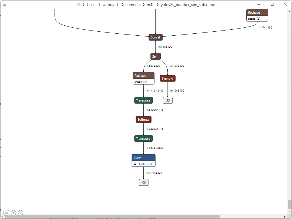
Extract the subgraph needed for inference (keep only the detection outputs):
import onnx

input_path = "/root/ultralytics/runs/detect/train17/weights/digit_yolov8s_sim.onnx"
output_path = "digit_yolov8s_sub.onnx"
input_names = ["images"]
output_names = ["400","433"]

onnx.utils.extract_model(input_path, output_path, input_names, output_names)
Preparing Quantization Resources
Create a directory structure for Pulsar2:
deploy_data/
├── config/
│   └── digit_config.json
├── dataset/
│   └── calibration_images.tar
├── model/
│   └── digit_yolov8s_sub.onnx
└── pulsar2-run-helper
The configuration file digit_config.json:
{
  "model_type": "ONNX",
  "npu_mode": "NPU1",
  "quant": {
    "input_configs": [
      {
        "tensor_name": "images",
        "calibration_dataset": "./dataset/calibration_images.tar",
        "calibration_size": 4,
        "calibration_mean": [0, 0, 0],
        "calibration_std": [255.0, 255.0, 255.0]
      }
    ],
    "calibration_method": "MinMax",
    "precision_analysis": true,
    "precision_analysis_method":"EndToEnd"
  },
  "input_processors": [
    {
      "tensor_name": "images",
      "tensor_format": "BGR",
      "src_format": "BGR",
      "src_dtype": "U8",
      "src_layout": "NHWC"
    }
  ],
  "output_processors": [
    {
      "tensor_name": "400",
      "dst_perm": [0, 1, 3, 2]
    },
    {
      "tensor_name": "433",
      "dst_perm": [0, 2, 1]
    }
  ],
  "compiler": {
    "check": 0
  }
}
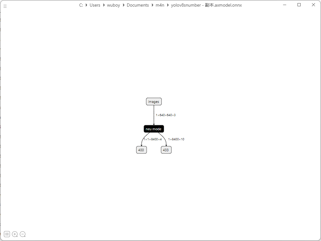
Generating the AXModel
Copy the deploy_data folder into the Pulsar2 Docker environment and execute quantization and compilation:
cd deploy_data/
pulsar2 build --input model/digit_yolov8s_sub.onnx --output_dir output --config config/digit_config.json
Extracts from the build log (trimmed for brevity):
...
Quant Config Table
┏━━━━━━━━┳━━━━━━━━━━━━━━━━━━┳━━━━━━━━━━━━━━━━━━━┳━━━━━━━━━━━━━┳━━━━━━━━━━━━━━━┳━━━━━━━━━━━━━━━━━┳━━━━━━━━━━━━━━━━━━━━━━━┓
┃ Input  ┃ Shape            ┃ Dataset Directory ┃ Data Format ┃ Tensor Format ┃ Mean            ┃ Std                   ┃
┡━━━━━━━━╇━━━━━━━━━━━━━━━━━━╇━━━━━━━━━━━━━━━━━━━╇━━━━━━━━━━━━━╇━━━━━━━━━━━━━━━╇━━━━━━━━━━━━━━━━━╇━━━━━━━━━━━━━━━━━━━━━━━┩
│ images │ [1, 3, 640, 640] │ images            │ Image       │ BGR           │ [0.0, 0.0, 0.0] │ [255.0, 255.0, 255.0] │
└────────┴──────────────────┴───────────────────┴─────────────┴───────────────┴─────────────────┴───────────────────────┘
...
Network Quantization Finished.
quant.axmodel export success: output/quant/quant_axmodel.onnx
...
max_cycle = 8,507,216
...
Rename the resulting quantized model for clarity:
mv output/quant/quant_axmodel.onnx digit_yolov8s.axmodel
Deploying to the AX650N Board
Using the 1.27 board image with local compilation. Clone the AX samples repository:
git clone https://github.com/AXERA-TECH/ax-samples.git
Inside ax_yolov8s_steps.cc, set the class labels and count for digit recognition:
const char* CLASS_NAMES[] = {
    "0", "1", "2", "3", "4", "5", "6", "7", "8", "9"};

int NUM_CLASS = 10;
Build the project:
cd ax-samples
mkdir build && cd build
cmake -DBSP_MSP_DIR=/soc/ -DAXERA_TARGET_CHIP=ax650 ..
make -j6
make install
The executables are installed under ax-samples/build/install/ax650/. Copy the digit_yolov8s.axmodel and a test image into that directory. Then run inference:
./ax_yolov8 -m digit_yolov8s.axmodel -i sample_digit.jpg
Example output:
--------------------------------------
model file : digit_yolov8s.axmodel
image file : sample_digit.jpg
img_h, img_w : 640 640
--------------------------------------
...
post process cost time:0.49 ms
Repeat 1 times, avg time 10.92 ms, max_time 10.92 ms, min_time 10.92 ms
--------------------------------------
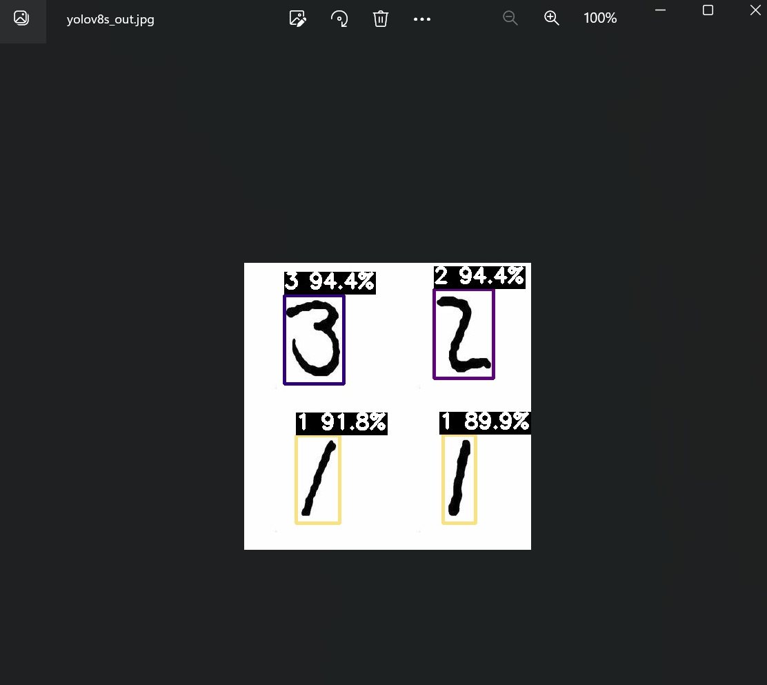
detection num: 4
2: 94%, [ 275, 38, 362, 168], 2
3: 94%, [ 58, 47, 145, 175], 3
1: 92%, [ 75, 250, 140, 378], 1
1: 90%, [ 288, 249, 336, 378], 1