Steps

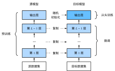
Below we introduce fine‑tuning, a common technique in transfer learning. As illustrated in the following diagram, fine‑tuning consists of four steps.

• Pre‑train a neural network model (the source model) on a source dataset, e.g., ImageNet.
• Create a new neural network (the target model). It replicates all model design and parameters from the source model, except the output layer. We assume these parameters contain knowledge learned from the source dataset that will also be useful for the target dataset. We also assume that the output layer of the source model is tightly coupled to the labels of the source dataset; therefore we do not use that layer in the target model.
• Add an output layer to the target model, whose number of outputs equals the number of categories in the target dataset, and randomly initialize the parameters of this added layer.
• Train the target model on the target dataset (e.g., a dataset of chairs). The output layer is trained from scratch, while all other layers have their parameters fine‑tuned based on the source model’s parameters.

When the target dataset is much smaller than the source dataset, fine‑tuning helps improve generalization.

Hotdog Recognition

Let us demonstrate fine‑tuning with a concrete example: hotdog recognition. We will fine‑tune a ResNet model, which was pre‑trained on the ImageNet dataset, on a small dataset containing thousands of images with and without hotdogs. We will use the fine‑tuned model to decide whether an image contains a hotdog.

%matplotlib inline
import os
import torch
import torchvision
import torch.nn as nn
from d2l import torch as d2l

Obtaining the Dataset

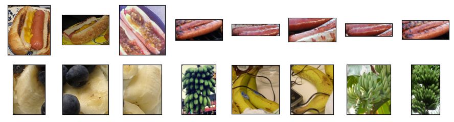
The hotdog dataset we use is collected from online sources. It contains 1400 positive‑class images of hotdogs, and as many negative‑class images of other foods. 1000 images of both classes are used for training, and the rest are used for testing.

After extracting the downloaded dataset, we obtain two folders hotdog/train and hotdog/test. Both folders have sub‑folders hotdog (with hotdog) and not-hotdog (without hotdog), each containing images of the corresponding class.

#@save
d2l.DATA_HUB['hotdog'] = (d2l.DATA_URL + 'hotdog.zip',
                         'fba480ffa8aa7e0febbb511d181409f899b9baa5')

data_dir = d2l.download_extract('hotdog')

Downloading ..\data\hotdog.zip from http://d2l-data.s3-accelerate.amazonaws.com/hotdog.zip...

We create two instances to read all image files from the training and test datasets.

train_data = torchvision.datasets.ImageFolder(os.path.join(data_dir, 'train'))
test_data = torchvision.datasets.ImageFolder(os.path.join(data_dir, 'test'))

The following displays the first 8 positive samples and the last 8 negative samples. As you can see, images vary in size and aspect ratio.

positive_samples = [train_data[i][0] for i in range(8)]
negative_samples = [train_data[-i - 1][0] for i in range(8)]
d2l.show_images(positive_samples + negative_samples, 2, 8, scale=1.4)

During training, we first crop a random region of random size and random aspect ratio from the image, then resize that region to \(224 \times 224\) and normalize it. The cropped region is used as input. During testing, we resize both height and width of an image to 256 pixels, then crop the central \(224 \times 224\) region as input. Additionally, for the RGB color channels we normalize each channel separately: subtract the channel mean and divide by the channel standard deviation.

# Use RGB channel means and standard deviations to normalize each channel
channel_norm = torchvision.transforms.Normalize(
    mean=[0.485, 0.456, 0.406],
    std=[0.229, 0.224, 0.225])

# Training data augmentations
train_transforms = torchvision.transforms.Compose([
    torchvision.transforms.RandomResizedCrop(224),
    torchvision.transforms.RandomHorizontalFlip(),
    torchvision.transforms.ToTensor(),
    channel_norm
])

# Testing data preprocessing
test_transforms = torchvision.transforms.Compose([
    torchvision.transforms.Resize([256, 256]),
    torchvision.transforms.CenterCrop(224),
    torchvision.transforms.ToTensor(),
    channel_norm
])

Defining and Initializing the Model

We use ResNet‑18 pre‑trained on ImageNet as the source model. Here we specify weights to automatically download the pre‑trained parameters. An internet connection is required if the model is being used for the first time.

pretrained_model = torchvision.models.resnet18(
    weights=torchvision.models.ResNet18_Weights.IMAGENET1K_V1)

The pre‑trained source model instance contains many feature layers and an output layer fc. This division is convenient for fine‑tuning all layers except the output layer. The member variable fc is shown below.

pretrained_model.fc

Linear(in_features=512, out_features=1000, bias=True)

After the global average pooling layer of ResNet, the fully connected layer outputs 1000 classes for the ImageNet dataset. Next, we construct a new neural network as the target model. Its defined in the same way as the pre‑trained source model, except that the number of outputs in the final layer is set to the number of classes in the target dataset (2 instead of 1000).

In the code below, the parameters of the member variable features in the target model fine_tune_model are initialized with the corresponding layer parameters of the source model. Because these parameters were pre‑trained on ImageNet and are good enough, usually only a small learning rate is needed to fine‑tune them.

The parameters of the newly added output layer are randomly initialized and typically require a higher learning rate to be trained from scratch. Let the learning rate of a Trainer instance be \(\eta\); we set the learning rate of the output layer parameters to \(10\eta\).

fine_tune_model = torchvision.models.resnet18(
    weights=torchvision.models.ResNet18_Weights.IMAGENET1K_V1)
fine_tune_model.fc = nn.Linear(fine_tune_model.fc.in_features, 2)
nn.init.xavier_uniform_(fine_tune_model.fc.weight)

Fine‑Tuning the Model

First, we define a training function fine_tune that implements fine‑tuning logic and can be called multiple times.

def fine_tune(net, lr, batch_size=128, num_epochs=5, use_fine_tune=True):
    train_dataset = torchvision.datasets.ImageFolder(
        os.path.join(data_dir, 'train'), transform=train_transforms)
    test_dataset = torchvision.datasets.ImageFolder(
        os.path.join(data_dir, 'test'), transform=test_transforms)

    train_loader = torch.utils.data.DataLoader(
        train_dataset, batch_size=batch_size, shuffle=True)
    test_loader = torch.utils.data.DataLoader(
        test_dataset, batch_size=batch_size)

    devices = d2l.try_all_gpus()
    criterion = nn.CrossEntropyLoss(reduction='none')

    if use_fine_tune:
        # Parameters of feature layers use base learning rate,
        # output layer uses lr * 10
        base_params = [p for n, p in net.named_parameters()
                       if n not in ['fc.weight', 'fc.bias']]
        optimizer = torch.optim.SGD(
            [{'params': base_params},
             {'params': net.fc.parameters(), 'lr': lr * 10}],
            lr=lr, weight_decay=0.001)
    else:
        optimizer = torch.optim.SGD(net.parameters(), lr=lr,
                                    weight_decay=0.001)

    d2l.train_ch13(net, train_loader, test_loader, criterion,
                   optimizer, num_epochs, devices)

We use a small learning rate to fine‑tune the pre‑trained parameters.

fine_tune(fine_tune_model, 5e-5)

loss 0.177, train acc 0.928, test acc 0.941
296.9 examples/sec on [device(type='cuda', index=0)]

For comparison, we define an identical model but initialize all its parameters randomly. Since the whole model must be trained from scratch, a larger learning rate is used.

scratch_model = torchvision.models.resnet18(weights=None)  # no pre‑training
scratch_model.fc = nn.Linear(scratch_model.fc.in_features, 2)
fine_tune(scratch_model, 5e-4, use_fine_tune=False)

loss 0.111, train acc 0.959, test acc 0.940
381.5 examples/sec on [device(type='cuda', index=0)]

As expected, the fine‑tuned model usually performs better because its initial parameter values are more effective.

Summary

• Transfer learning moves knowledge learned from a source dataset to a target dataset; fine‑tuning is a common transfer learning technique.
• Except for the output layer, the target model copies all model designs and parameters from the source model, and fine‑tunes these parameters. The output layer of the target model must be trained from scratch.
• Typically, fine‑tuned parameters use a smaller learning rate, while the output layer trained from scratch can use a larger learning rate.