During a recent internship in the OTC derivatives department of a securities firm, I worked on a project involving delta dynamic hedging for pricing vanilla options. Referencing John Hull's Options, Futures, and Other Derivatives, which covers delta hedging, I used Python to replicate the book's examples.

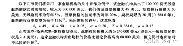
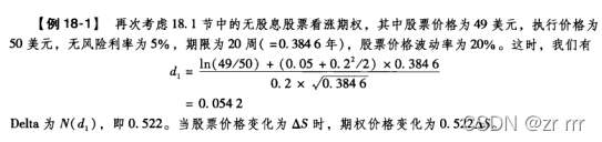
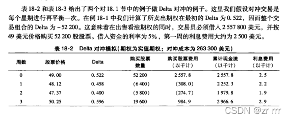
To hedge the risk of a sold call option, one must buy a certain number of shares. The number of shares purchased equals the call option's delta multiplied by the number of options sold. In this example, delta is 0.522.

The following sections show two hedging scanarios, corresponding to whether the option expires in the money or out of the money.

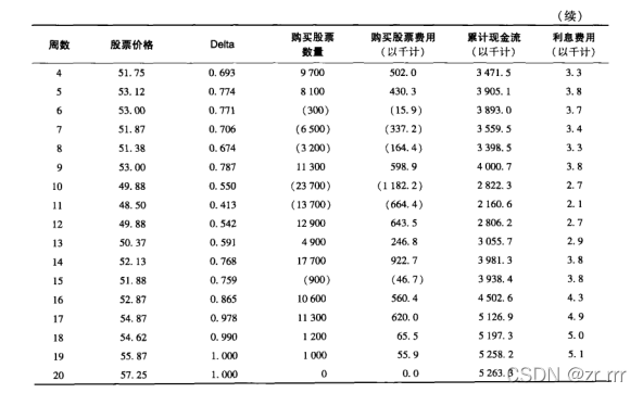
Scenario 1: The stock price at expiration is above the strike price, allowing exercise. The replication cost of the option is $263,300.

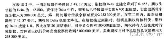
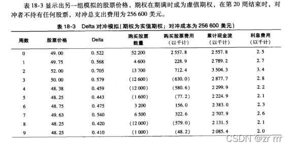
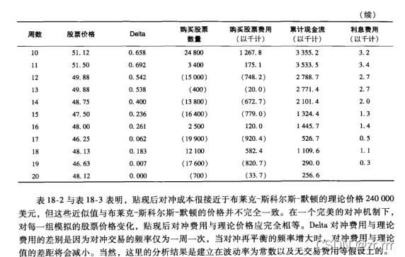
Scenario 2: The stock price at expiration is below the strike price, so the option expires worthless. The replication cost is $256,600.

Python Implementation

First, define a module bsm.py that calculates the value and delta of a call option under the Black-Scholes-Merton model.

from math import log, sqrt, exp
from scipy import stats
import numpy as np

class BSMOptionValuation:
    def __init__(self, S0, K, T, r, sigma, div=0.0):
        self.S0 = float(S0)
        self.K = float(K)
        self.T = float(T)
        self.r = float(r)
        self.sigma = float(sigma)
        self.div_yield = float(div)
        self.d1 = ((log(self.S0 / self.K) + (self.r - self.div_yield + 0.5 * self.sigma ** 2) * self.T) / (self.sigma * sqrt(self.T)))
        self.d2 = self.d1 - self.sigma * sqrt(self.T)

    def call_value(self):
        return (self.S0 * exp(-self.div_yield * self.T) * stats.norm.cdf(self.d1, 0.0, 1.0) - self.K * exp(-self.r * self.T) * stats.norm.cdf(self.d2, 0.0, 1.0))

    def delta(self):
        delta_call = exp(-self.div_yield * self.T) * stats.norm.cdf(self.d1, 0.0, 1.0)
        delta_put = -exp(-self.div_yield * self.T) * stats.norm.cdf(-self.d1, 0.0, 1.0)
        return delta_call, delta_put

Then, replicate the case study. The following code uses the first stock price path (results match the book). You can test with the second path for verification.

from math import log, sqrt, exp
import numpy as np
import scipy.stats as si
from scipy.stats import norm
from bsm import BSMOptionValuation
import pandas as pd

if __name__ == '__main__':
    # Option parameters
    N = 100000                          # Number of options
    S1 = [49, 48.12, 47.37, 50.25, 51.75, 53.12, 53, 51.87, 51.38, 53, 49.88, 48.5, 49.88, 50.37, 52.13, 51.88, 52.87, 54.87, 54.62, 55.87, 57.25]  # Stock price path 1
    S2 = [49, 49.75, 52, 50, 48.38, 48.25, 48.75, 49.63, 48.25, 48.25, 51.12, 51.5, 49.88, 49.88, 48.75, 47.5, 48, 46.25, 48.13, 46.63, 48.12]  # Stock price path 2
    K = 50                              # Strike price
    r = 0.05                            # Risk-free rate
    sigma = 0.2                         # Volatility
    T = 0.3846                          # Time to maturity (years)
    simulation = 20                     # Number of steps in the path
    dt = T / simulation                 # Time step size

    # Initialize structures
    expire_time = np.append((np.ones((simulation, 1)) * dt).cumsum()[::-1], 0)  # Remaining time to expiration
    cash = np.zeros(simulation + 1)                                             # Cash account
    div = np.zeros(simulation)                                                 # Interest earned on cash
    delta = np.zeros(simulation)                                               # Delta values

    # Hedging loop
    for step in range(simulation + 1):
        if step == 0:  # Initial position
            delta[step] = BSMOptionValuation(S1[step], K, expire_time[step], r, sigma).delta()[0]
            cash[step] = delta[step] * N * S1[0]  # Cash required to buy delta shares
            div[step] = cash[step] * r * dt
        elif step < simulation:  # Rebalancing steps
            delta[step] = BSMOptionValuation(S1[step], K, expire_time[step], r, sigma).delta()[0]
            cash[step] = cash[step-1] + div[step-1] + (delta[step] - delta[step-1]) * S1[step] * N
            div[step] = cash[step] * r * dt
        else:  # Settlement at expiration
            if S1[step] > K:
                cash[step] = cash[step-1] + div[step-1] - N * K
            else:
                cash[step] = cash[step-1] + div[step-1] - delta[step-1] * S2[step] * N

    print(cash[-1])  # Option replication cost

Output for scenario 1:

263061.29677824676

This result closely matches the book's value of $263,300. The small discrepancy arises because the book rounds intermediate calculations to one decimal place. The result for the second stock price path is:

256520.06138881645

This is very close to the book's $256,600.

Next Steps

In practice, industry often uses cash delta rather than standard delta for dynamic hedging. Additionally, stock price paths can be simulated via Monte Carlo methods. The next article will demonstrate how to implement cash delta dynamic hedging using Monte Carlo simulation in Python.