Logistic Function

Logistic regression is a generalized linear model, sharing many similarities with multiple linear regression.

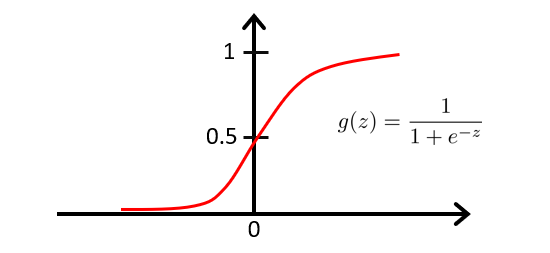
We define the logistic function (sigmoid) as:

$$ g(z) = \frac{1}{1 + e^{-z}} $$

With $ z = \theta^T x $, the hypothesis becomes:

$$ h_\theta(x) = \frac{1}{1 + e^{-\theta^T x}} $$

The graph of the logistic function is:

When we have $ h_\theta(x) $, we need to fit parameters $ \theta $ to the data, similar to linear regression.

Since the logistic function outputs values between 0 and 1, and the prediction is either 0 or 1, $ h_\theta(x) $ represents the probability of predicting 1. For example, if $ h_\theta(x) = 0.7 $, then:

$$ P(y=1|x,\theta) = 0.7 $$ $$ P(y=0|x,\theta) = 0.3 $$

Decision Boundary

We can set a threshold, e.g., 0.5, to decide the class:

• If $ h_\theta(x) \geq 0.5 $, predict $ y=1 $
• If $ h_\theta(x) < 0.5 $, predict $ y=0 $

From the sigmoid graph:

• When $ z \geq 0 $, $ h_\theta(x) \geq 0.5 $
• When $ z < 0 $, $ h_\theta(x) < 0.5 $

Consider a training set and hypothesis:

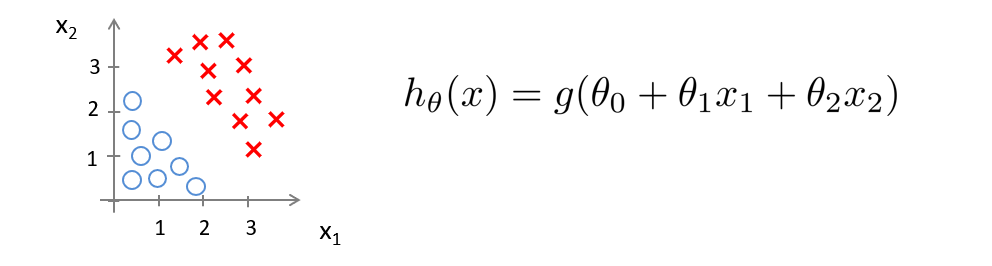
Let $ \theta_0 = -3, \theta_1 = 1, \theta_2 = 1 $.

Then if $ -3 + x_1 + x_2 \geq 0 $, predict $ y=1 $. This defines a linear decision boundary:

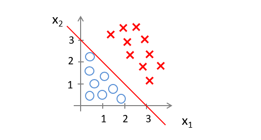
Points to the right of the line are classified as 1, to the left as 0.

Another example:

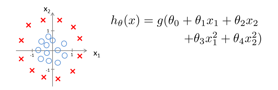
With $ \theta_0 = -1, \theta_1 = 0, \theta_2 = 0, \theta_3 = 1, \theta_4 = 1 $, the condition becomes $ -1 + x_1^2 + x_2^2 \geq 0 $, giving a circular decision boundary:

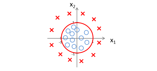
The decision boundary is determined by the parameters $ \theta $, not the training set.

Cost Function

Given a training set with $ n $ features and $ m $ samples, we set $ x_0 = 1 $.

Hypothesis:

$$ h_\theta(x) = \frac{1}{1 + e^{-\theta^T x}} $$

In linear regression, the cost function was:

$$ J(\theta) = \frac{1}{m} \sum_{i=1}^m \frac{1}{2} (h_\theta(x^{(i)}) - y^{(i)})^2 $$

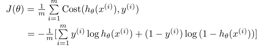
Define $ Cost(h_\theta(x^{(i)}), y^{(i)}) = \frac{1}{2} (h_\theta(x^{(i)}) - y^{(i)})^2 $, so $ J(\theta) = \frac{1}{m} \sum_{i=1}^m Costt(h_\theta(x^{(i)}), y^{(i)}) $.

For logistic regression, using the squared error results in a non-convex cost function with many local minima, so we define a different cost:

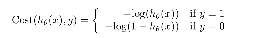
For $ y=1 $:

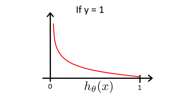
• If $ h_\theta(x) = 1 $, cost = 0
• If $ h_\theta(x) \to 0 $, cost $ \too \infty $

For $ y=0 $:

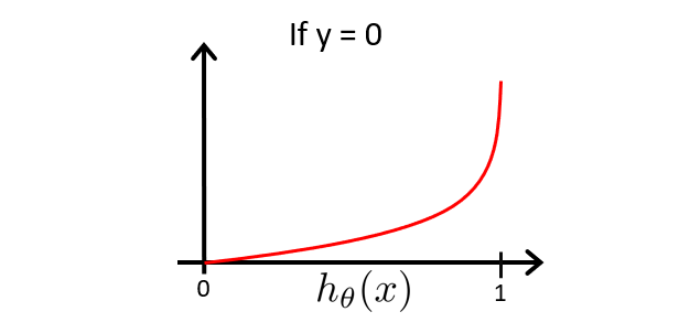
• If $ h_\theta(x) = 0 $, cost = 0
• If $ h_\theta(x) \to 1 $, cost $ \to \infty $

We can combine the two cases into one equation:

$$ Cost(h_\theta(x), y) = -y \log(h_\theta(x)) - (1-y) \log(1 - h_\theta(x)) $$

Thus the logistic regression cost function becomes:

Gradient Descent

To minimize $ J(\theta) $, we use gradient descent:

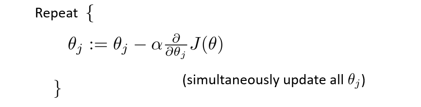
After computing the derivative, the update rule is:

$$ \theta_j := \theta_j - \alpha \frac{1}{m} \sum_{i=1}^m (h_\theta(x^{(i)}) - y^{(i)}) x_j^{(i)} $$

Multiclass Classification (One-vs-All)

For three classes:

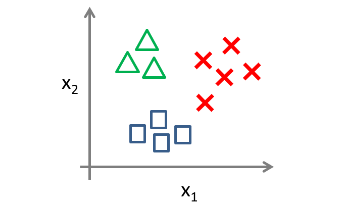
We can transform into three binary classification problems:

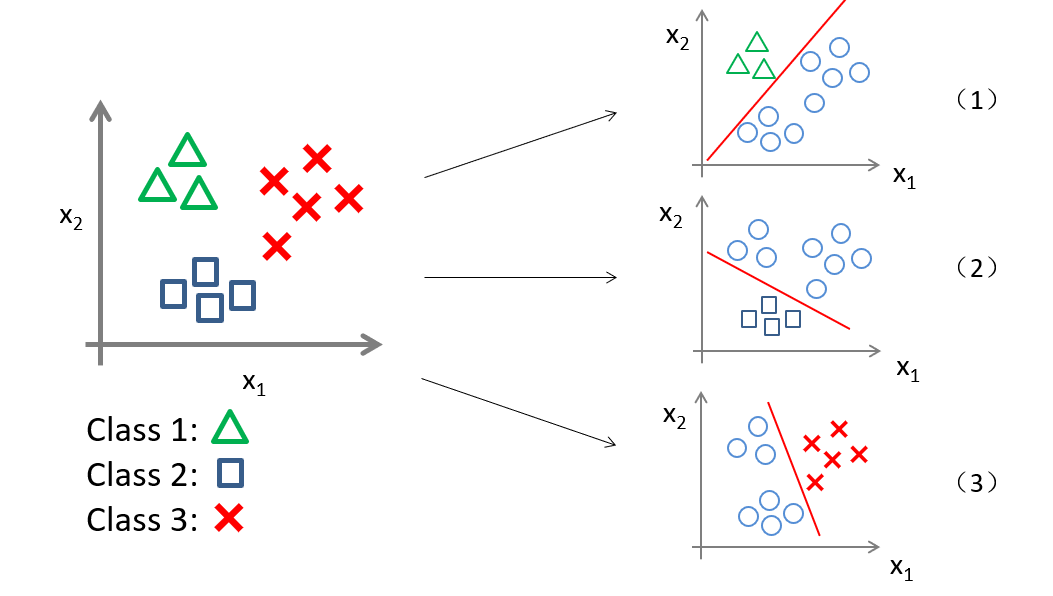
Each classifier predicts the probability for one class (e.g., $ y=1, y=2, y=3 $).

Overfitting and Regularization

Overfitting occurs when a hypothesis fits the training data well but fails on new data, often due to noise or insufficient data.

Solutions:

1. Reduce the number of features (manually or via model selection).
2. Regularization: keep all features but reduce the magnitude of parameters $ \theta $.

Modify the cost function:

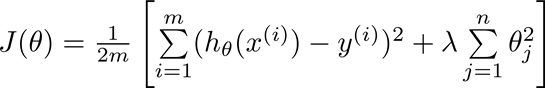
$ \lambda $ is the regularization parameter controlling the trade-off between fitting the data and keeping parameters small.

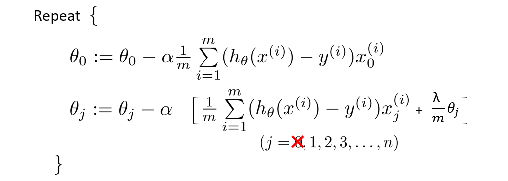
Regularized Linear Regression

Do not regularize $ \theta_0 $. Update rules:

Simplify:

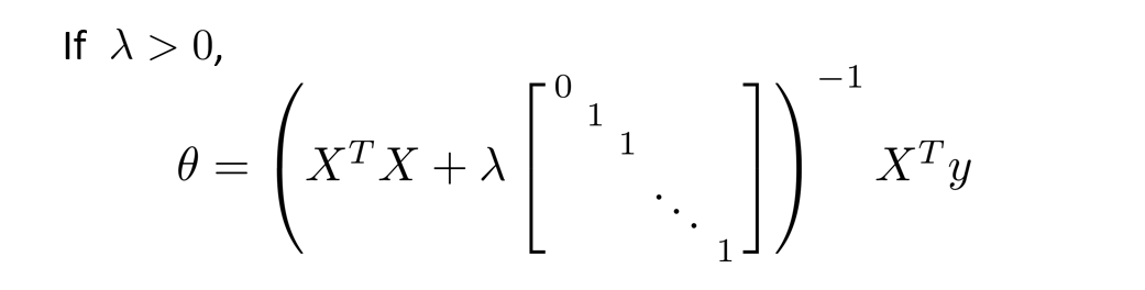
Normal equation becomes:

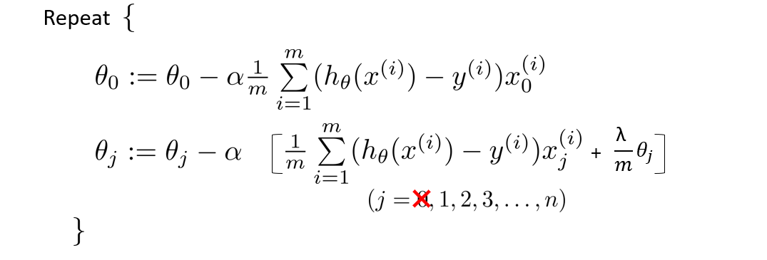
Regularized Logistic Regression

Example Code

import numpy as np
import pandas as pd
import matplotlib.pyplot as plt
from sklearn.metrics import classification_report

Linear Classification

# Load data
df = pd.read_csv('ex2data1.txt', names=['exam1', 'exam2', 'admitted'])
df.head()

# Summary statistics
df.describe()

# Scatter plot
admitted = df[df['admitted'] == 1]
not_admitted = df[df['admitted'] == 0]

plt.figure(figsize=(12,8))
plt.scatter(admitted.exam1, admitted.exam2, c='b', marker='o', label='Admitted')
plt.scatter(not_admitted.exam1, not_admitted.exam2, c='r', marker='x', label='Not Admitted')
plt.xlabel('Exam 1 Score')
plt.ylabel('Exam 2 Score')
plt.legend()

# Sigmoid function
def sigmoid(z):
    return 1 / (1 + np.exp(-z))

# Verify sigmoid
x = np.arange(-10, 10, 0.1)
plt.plot(x, sigmoid(x), 'r')
plt.title('Sigmoid Function')

Cost function:

# Add intercept term
df.insert(0, 'Ones', 1)

# Extract features and target
cols = df.shape[1]
X = np.array(df.iloc[:, 0:cols-1])
y = np.array(df.iloc[:, cols-1:cols])
params = np.zeros(3)

def compute_cost(params, X, y):
    params = np.matrix(params)
    X = np.matrix(X)
    y = np.matrix(y)
    m = len(X)
    h = sigmoid(X * params.T)
    cost = (1/m) * np.sum((-y).T * np.log(h) - (1-y).T * np.log(1 - h))
    return cost

Gradient:

def gradient(params, X, y):
    params = np.matrix(params)
    X = np.matrix(X)
    y = np.matrix(y)
    m = len(X)
    h = sigmoid(X * params.T)
    return (X.T * (h - y)) / m

Optimization with scipy:

import scipy.optimize as opt
result = opt.fmin_tnc(func=compute_cost, x0=params, fprime=gradient, args=(X, y))
optimal_params = result[0]
final_cost = compute_cost(optimal_params, X, y)
print(f'Optimal cost: {final_cost}')

Prediction function:

def predict(params, X):
    params = np.matrix(params)
    X = np.matrix(X)
    prob = sigmoid(X * params.T)
    return (prob >= 0.5).astype(int)

Evaluate:

y_pred = predict(optimal_params, X)
print(classification_report(y, y_pred))

Decision boundary:

# Coefficients for boundary: theta0 + theta1*x1 + theta2*x2 = 0
# Solve for x2: x2 = - (theta0 + theta1*x1)/theta2
coeff = -(optimal_params / optimal_params[2])
x_vals = np.arange(130, step=0.1)
y_vals = coeff[1] * x_vals + coeff[0]

plt.figure(figsize=(12,8))
plt.scatter(admitted.exam1, admitted.exam2, c='b', marker='o', label='Admitted')
plt.scatter(not_admitted.exam1, not_admitted.exam2, c='r', marker='x', label='Not Admitted')
plt.plot(x_vals, y_vals, 'purple', label='Decision Boundary')
plt.xlim(0, 120)
plt.ylim(0, 120)
plt.xlabel('Exam 1')
plt.ylabel('Exam 2')
plt.legend()

Non-linear Classsification with Regularization

df2 = pd.read_csv('ex2data2.txt', names=['test1', 'test2', 'accepted'])
df2.head()

# Scatter plot
accepted = df2[df2['accepted'] == 1]
rejected = df2[df2['accepted'] == 0]

plt.figure(figsize=(12,8))
plt.scatter(accepted.test1, accepted.test2, c='b', marker='o', label='Accepted')
plt.scatter(rejected.test1, rejected.test2, c='r', marker='x', label='Rejected')
plt.xlabel('Test 1')
plt.ylabel('Test 2')
plt.legend()

Feature mapping:

def feature_mapping(x1, x2, power, as_ndarray=False):
    data = {}
    for i in range(power + 1):
        for p in range(i + 1):
            data[f'f{i-p}{p}'] = np.power(x1, i-p) * np.power(x2, p)
    if as_ndarray:
        return pd.DataFrame(data).values
    else:
        return pd.DataFrame(data)

x1 = np.array(df2.test1)
x2 = np.array(df2.test2)
X_mapped = feature_mapping(x1, x2, power=6, as_ndarray=True)
y2 = np.array(df2.iloc[:, -1:])  # last column
params2 = np.zeros(28)

Regularized cost:

def regularized_cost(params, X, y, lam=1):
    # Exclude theta0 from regularization
    theta_reg = params[1:]
    reg = (lam / (2 * len(X))) * np.sum(theta_reg**2)
    return compute_cost(params, X, y) + reg

Regularized gradient:

def regularized_gradient(params, X, y, lam=1):
    theta_reg = params[1:]
    reg_term = (lam / len(X)) * theta_reg
    # Combine with zero for theta0
    reg_term = np.concatenate([np.array([0]), reg_term])
    return gradient(params, X, y) + reg_term.reshape(-1,1)

Optimization:

result2 = opt.fmin_tnc(func=regularized_cost, x0=params2, fprime=regularized_gradient, args=(X_mapped, y2))
optimal_params2 = result2[0]

Prediction and evaluation:

y_pred2 = predict(optimal_params2, X_mapped)
print(classification_report(y2, y_pred2))

Decision boundary for non-linear:

def find_decision_boundary(power, theta):
    t1 = np.linspace(-1, 1.5, 1000)
    t2 = np.linspace(-1, 1.5, 1000)
    coordinates = [(x, y) for x in t1 for y in t2]
    x_cord, y_cord = zip(*coordinates)
    mapped = feature_mapping(np.array(x_cord), np.array(y_cord), power)
    inner_product = mapped @ theta
    # Find points where inner_product is close to 0
    idx = np.abs(inner_product) < 0.001
    return mapped.iloc[:, 0][idx], mapped.iloc[:, 1][idx]

x_bound, y_bound = find_decision_boundary(6, optimal_params2)
plt.figure(figsize=(12,8))
plt.scatter(accepted.test1, accepted.test2, c='b', marker='o', label='Accepted')
plt.scatter(rejected.test1, rejected.test2, c='r', marker='x', label='Rejected')
plt.scatter(x_bound, y_bound, c='purple', s=1, label='Decision Boundary')
plt.xlabel('Test 1')
plt.ylabel('Test 2')
plt.legend()