Important Links
- matplotlib: matplotlib — Matplotlib 3.5.1 documentation
- seaborn: seaborn.lineplot — seaborn 0.13.2 documentation
- DataFrame: DataFrame — pandas 2.2.1 documentation
- Python Matplotlib Scatter, Line, Box, Bar Plot Examples: Python Matplotlib 实现散点图、曲线图、箱状图、柱状图示例
- Color Palettes: matplotlib、seaborn颜色、调色板、调色盘
Common Functions
Basic Operations
| Operation | Code |
|---|---|
| Get all column names | list(df), df.columns.tolist(), list(df.columns) |
| Get data type | type(df) (e.g., <class 'pandas.core.frame.DataFrame'>) |
| Get column types | df.dtypes |
| Uninstall package in Jupyter | !pip uninstall package_name -y |
| Convert ipynb to py in Jupyter | import nbconvert then !jupyter nbconvert --to script *.ipynb |
| Check version | package_name.__version__ |
| Change shape with numpy | pre = pre[:, np.newaxis] (e.g., from (300,) to (300,1)) |
| Append dataframes | df = df1.append(df2.append(df3)) |
| Compute quotient and remainder | div, mod = divmod(df['num'], n) |
| Print usage | print("Center is:", center) or print(f"Center is: {center}") |
Pandas loc and iloc
# loc: index by labels/names
# iloc: index by integer positions

# Sample data:
      AA  BB  CC  DD  EE
row1   2   3  56  55   4
row2   5   7   4  34   5
row3   9   7   4   7  15
row4   5  72  43  34   5

# loc examples
data1 = data.loc['row2']          # row2 data
data1 = data.loc['row2', :]       # same as above
data2 = data.loc[:, 'BB']         # column BB
data3 = data.loc['row1', 'BB']    # value 3
data4 = data.loc['row2':'row3', 'AA':'DD']  # rows 2-3, columns AA-DD
data5 = data.loc[data.BB > 6]     # rows where BB > 6
data6 = data.loc[data.BB > 6, ['BB', 'CC', 'DD']]  # subset

# iloc examples
data1 = data.iloc[1]              # second row
data1 = data.iloc[1, :]           # same
data2 = data.iloc[:, 1]           # second column
data3 = data.iloc[1, 1]           # row 2, column 2
data4 = data.iloc[1:3, 2:4]       # rows 2-3, columns 3-4 (0-indexed)
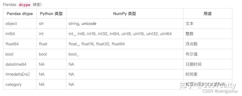
Data Types in Python, NumPy, and Pandas
Python's str and NumPy's string/unicode are rperesented as object in Pandas. Strings in Pandas are of type object.
datetime Conversion
import pandas as pd

# Convert object to datetime
df = pd.DataFrame({'date': ['2011-04-24 01:30:00.000']})
df['date'] = pd.to_datetime(df['date'])
# Result: 0   2011-04-24 01:30:00
# Name: date, dtype: datetime64[ns]

# Convert back to object
df['date'] = df['date'].astype('object')
# Result: same appearance but dtype: object

# Custom format
pd.to_datetime("20110424 01:30:00.000", format='%Y%m%d %H:%M:%S.%f')
Resampling with resample()
- Frequency: Python Time Series Resampling
- Algorithms: Pandas Resampling Documentation
# Fill missing time at 1-minute intervals, fill NaN with forward fill
# ffill() uses previous value, interpolate() uses interpolation, bfill() uses next value
df = df.resample('1T').mean().ffill()

# Get 5-minute intervals
# asfreq() or other methods like first()
df5 = df.resample('5T').asfreq()
# Alternative
df5 = df.loc[::5, :]
set_index()
df.set_index(keys, drop=True, append=False, inplace=False, verify_integrity=False)
# keys: column label or list of labels to become index
# drop: if True, remove the column used as index (default True)
# append: if True, append to existing index (default False)
# inplace: if True, modify the original DataFrame (default False)
# verify_integrity: check for duplicates (default False)
reset_index()
# Convert index back to a column
df.reset_index(drop=False, inplace=False, level=None, col_level=0, col_fill='')
# drop: if True, do not insert the old index as a column (default False)
# inplace: if True, modify the original DataFrame (default False)
# level: if MultiIndex, remove only specified level(s)
# col_level, col_fill: for MultiIndex columns
import pandas as pd
import numpy as np
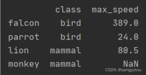
df = pd.DataFrame([('bird', 389.0), ('bird', 24.0), ('mammal', 80.5), ('mammal', np.nan)],
index=['falcon', 'parrot', 'lion', 'monkey'],
columns=['class', 'max_speed'])
# Original
print(df)
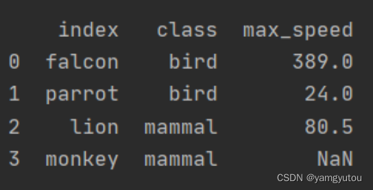
# Reset with index becoming a column
df1 = df.reset_index()
print(df1)
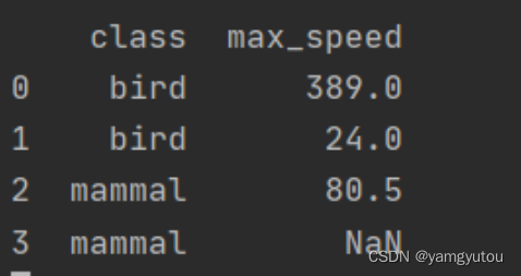
# Reset and drop index
df2 = df.reset_index(drop=True)
print(df2)
Timing Execution
import time
start_time = time.time()
# your code here
end_time = time.time()
execution_time = end_time - start_time
rename()
# Rename columns and/or index
df.rename(columns={'old_col': 'new_col'}, index={'old_idx': 'new_idx'}, inplace=False)
# Alternatively, use axis parameter
# axis='index' for row labels, axis='columns' for column labels

import pandas as pd
df = pd.DataFrame({'A': [1,2,3], 'B': [4,5,6]})

# Rename columns without axis
df.rename(columns={'A': 'a', 'B': 'c'})
# Returns new DataFrame; original unchanged (inplace=False by default)

# Rename rows and columns simultaneously
df_re = df.rename(columns={'A': 'a', 'B': 'c'}, index={0: '0a', 1: '1a'})
print(df_re)

# Using axis
# Rename rows with axis='index'
df.rename({1: 2, 2: 4}, axis='index')
# Rename columns with axis='columns'
df.rename(str.lower, axis='columns')
Plotting Functions
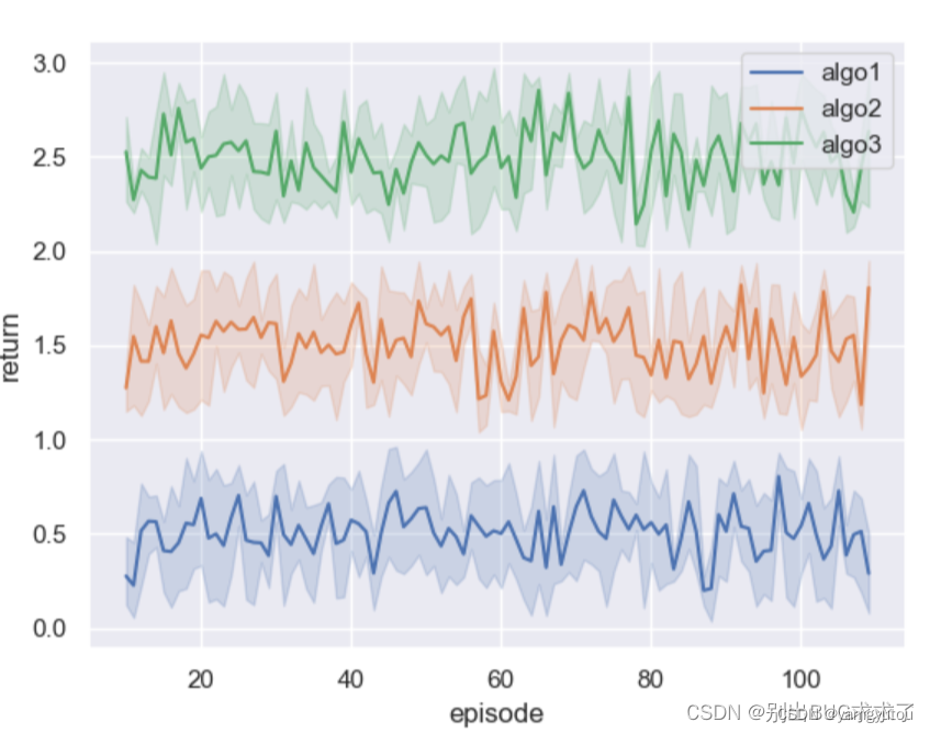
Mean and Standard Deviation Shaded Plot
Plotting mean and standard deviation with seaborn
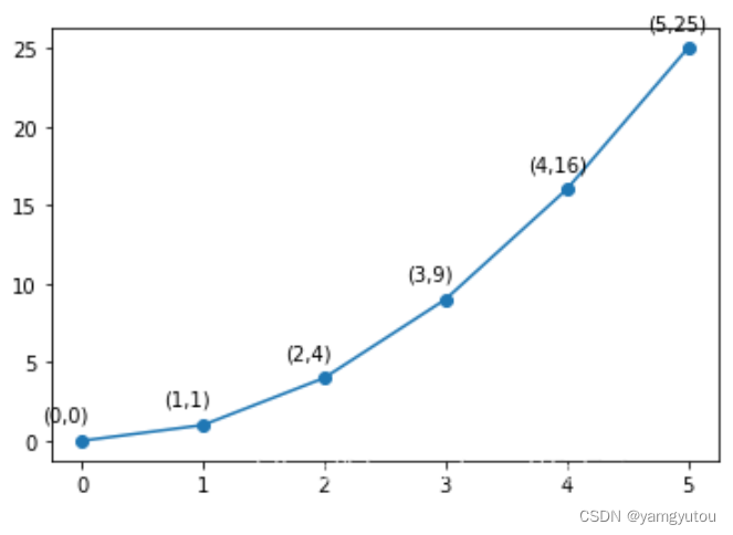
plt.annnotate()
Used to annotate specific points on a plot, typically in a loop.
Reference: matplotlib.pyplot.annotate
import matplotlib.pyplot as plt
import numpy as np
x = np.arange(0, 6)
y = x * x
# Simple annotation on each point
plt.plot(x, y, marker='o')
for xi, yi in zip(x, y):
plt.annotate(f"({xi},{yi})", xy=(xi, yi), xytext=(-20, 10), textcoords='offset points')
plt.show()
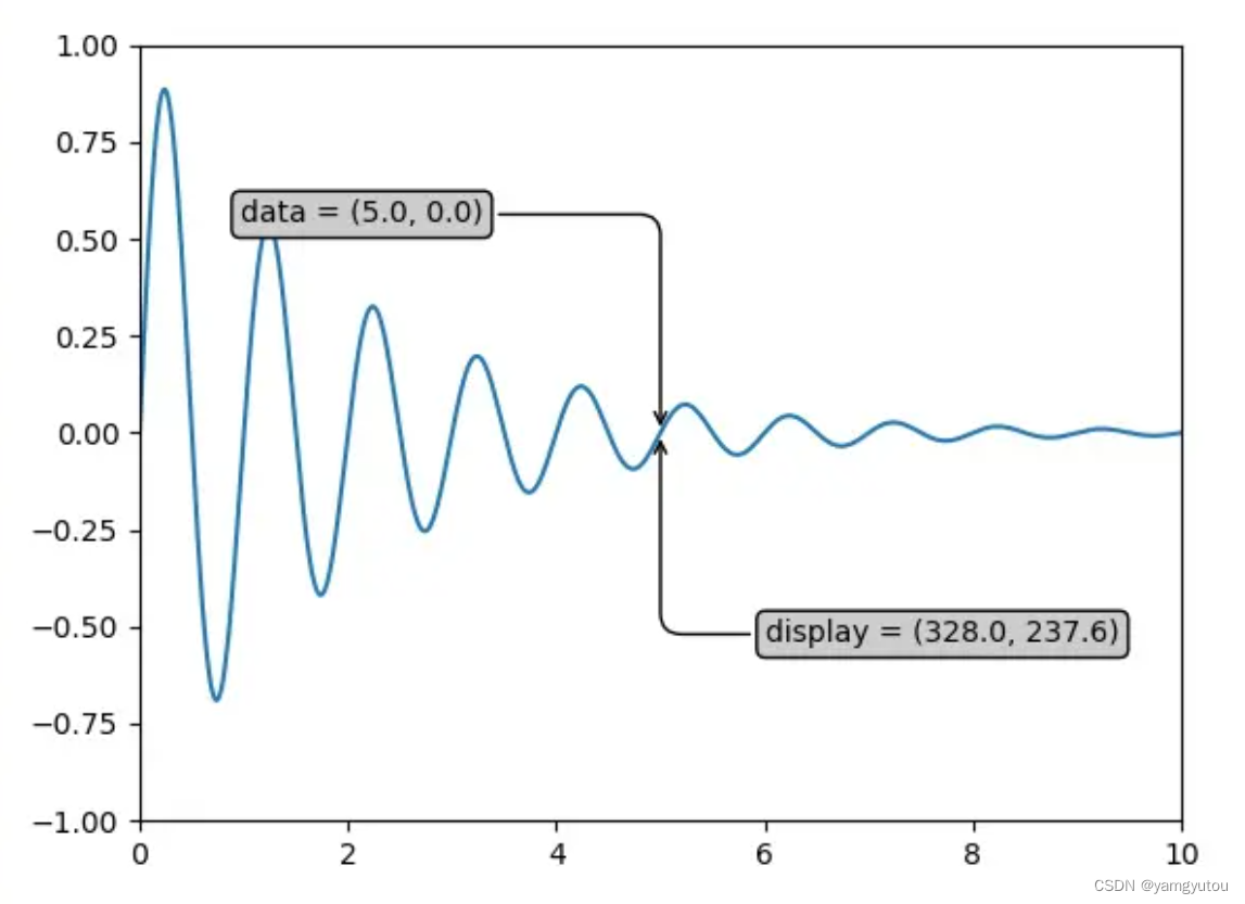
# More advanced annotation with box and arrow
bbox = dict(boxstyle='round,pad=0.3', facecolor='yellow', alpha=0.5)
arrowprops = dict(arrowstyle='->', connectionstyle='arc3,rad=0')
ax.annotate(f'data = ({xi:.1f}, {yi:.1f})',
(xi, yi), xytext=(-2*10, 10), textcoords='offset points',
bbox=bbox, arrowprops=arrowprops)
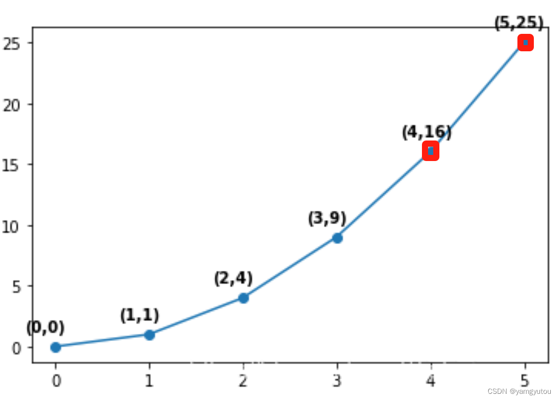
# Combine with scatter to highlight specific points
x1, y1 = [], []
plt.plot(x, y, marker='o')
for xi, yi in zip(x, y):
if xi > 3:
plt.annotate(f"({xi},{yi})", xy=(xi, yi), xytext=(-20, 10), textcoords='offset points')
x1.append(xi)
y1.append(yi)
plt.scatter(x1, y1, marker='p', color='m')
plt.show()